How to Measure Cannabis Light: PAR Meters, Phone Apps, PPFD Maps, and Canopy Grids
A grow light can look bright while delivering very different photon levels to the center, edges, and tallest flowers. Its published PPFD chart might have been measured at a different hanging height, inside a different enclosure, or across a footprint larger than the area occupied by your plants. The useful measurement is not the brightest spot beneath the fixture. It is a documented set of readings across the canopy you actually intend to illuminate.
For a conventional plant-light measurement, use photosynthetic photon flux density (PPFD) in µmol/m²/s. Define the measurement surface, place an appropriate sensor at repeatable positions, record the light settings, and calculate the average alongside low and high readings. Then change one lighting variable and repeat the same grid. This approach exposes weak corners, central hotspots, overlap between fixtures, and changes caused by plant growth that a single center reading would miss.
A calibrated quantum sensor is the defensible choice when absolute PPFD matters. A correctly configured phone application may help with relative checks or a preliminary map, but its accuracy depends on the device, optical setup, calibration, and light spectrum. A manufacturer’s map is valuable design information, not a substitute for installed measurements. This resource explains how to collect a credible map, interpret it, and verify any correction. For the broader lamp-selection background, see the cannabis grow light guide; stage-specific light targets and comprehensive DLI calculations remain separate subjects.
Build a Repeatable Canopy Measurement Grid
Before taking the first reading, decide what surface you are trying to describe. A PPFD map is a description of photon flux at a defined plane under a defined lighting condition. Change the plane, footprint, wall reflectance, or fixture setting and the map becomes a different experiment. Write down the boundaries and height first; the meter comes second.
Start with the actual occupied growing footprint, not automatically the entire tent floor. A 120 × 120 cm enclosure holding plants over a central 90 × 90 cm area has two legitimate questions: how evenly the existing plants are lit and whether a future full-footprint canopy would be lit evenly. Map these as separate footprints rather than inflating one average with unplanted perimeter cells or excluding weak edges to make an installed fixture look better.
Measure the intended plant surface length and width and draw a rectangle. Mark its corners, the fixture centerline, and any seam between fixtures. Record whether your footprint is the planted canopy, a planned flowering footprint, a propagation tray, or an empty design plane. The geometry must be identical when you compare before and after readings.
Divide the rectangle into equal-area cells and measure at each cell center. A 3 × 3 grid gives nine readings and is useful for a compact preliminary survey. A 5 × 5 grid gives 25 readings and is better at revealing spatial patterns across a modest, regular footprint. Larger commercial areas, narrow fixtures, strong hotspots, irregular canopies, or complex fixture overlap may need tighter spacing and additional diagnostic points. There is no universal nine-point or 25-point rule; choose a resolution fine enough for the variation you need to see.
For example, divide a 100 × 100 cm footprint into five equal rows and five equal columns. Each cell is 20 × 20 cm, and its center falls at 10, 30, 50, 70, or 90 cm along either axis. Record the crossing of each x and y center, resulting in 25 equal-area observations. This cell-center method estimates the area-average PPFD without treating a corner and the center as if each represented the same surrounding area.
For a different purpose, you may put readings exactly at the boundaries, corners, or directly beneath fixture bars. Label those as supplementary diagnostic points, not extra equal-area samples in the mean. If you combine many closely spaced hotspot measurements with a small number of edge measurements and take their simple average, you have biased the average toward the region you sampled more heavily.
Field Advice: Mark the x and y positions on a rigid board, measuring tape, or annotated floor plan before you begin. The board is a location guide, not a platform that should shade or raise the sensor. Repeatable coordinates are more valuable than a beautifully colored map made from unrepeatable hand positions.
Choose one canopy plane and document exceptions
For a relatively level canopy under overhead lighting, choose a horizontal plane representing the tops of the productive foliage. State its distance below a fixed reference such as a ceiling rail, tent crossbar, or luminaire mounting surface. A statement such as “30 cm below the light” is incomplete if one fixture has a deeper housing, a hanging driver, or multiple emitting bars. Identify the reference surface and measure it the same way later.
Live cannabis canopies are rarely perfectly flat. If the tallest cola sits 20 cm above most of the canopy, moving the meter up and down at every grid cell measures different planes and confounds your map. First make a single-plane map at the representative top-canopy height. Then take separately labeled readings at unusually tall flowers, low branches, deep interior positions, or propagation trays when those surfaces present a distinct plant-risk question. A horizontal grid is not a complete three-dimensional light profile.
Where branches obstruct access, use a clean rigid extension or dedicated sensor wand to reach the designated point without bending delicate flowers or casting shadows. Do not flatten plants to make a laboratory-like surface and then assume the map describes their undisturbed growing condition. If the canopy cannot be reached safely, use a nearby accessible plane and state that limitation rather than reporting the substitute as the exact flower-top exposure.
Control fixture warm-up, dimming, photoperiod, and room state
Measure with the lights operating in the state you want to evaluate. Record fixture count, arrangement, hanging height, output setting, channel configuration, and whether the timer is in a normal full-output period or a programmed ramp. Some lighting systems change output as they warm up, while others are stable quickly. Follow the equipment instructions and confirm that repeated readings at one reference point have stopped drifting within your measurement tolerance. Do not claim a universal warm-up time for every LED or HID fixture.
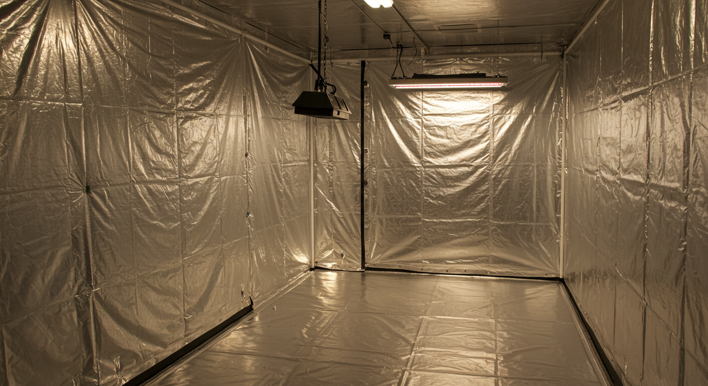
Keep the doors, reflective walls, curtains, neighboring lamps, and ventilation configuration as they normally are for the intended test. An open tent door can change reflection. A person leaning into a small tent can shade the sensor. Moving a white board into the room for easy positioning can alter the light field. Record and control such changes. Avoid looking directly into high-intensity LEDs or touching hot fixtures. Keep handheld meters and phone devices away from irrigation spray and wet electrical connections.
Prepare a blank grid with labeled rows and columns. Confirm the correct PPFD measurement mode and waveband. Clean and level the sensor according to its manual, choose the reference plane, stabilize the lighting, and note one fixed reference-point reading. Move through the cells in an organized route, holding the sensor at the same height and orientation. Wait for the display or logger to settle where necessary, then record the actual value and units in its correct cell. Return to the reference point at the end. A different final reading under supposedly unchanged conditions is a reason to check output drift, shadows, accidental dimmer movement, or instrument behavior before interpreting the grid.
If the environment is changing, especially when sunlight contributes, a full grid collected over many minutes may mix time variation with position variation. Log a fixed reference sensor during the survey, measure more quickly in stable periods, or repeat positions in a balanced order. In a greenhouse, a measurement at the west edge at 09:00 cannot be directly compared with an east-edge measurement at 10:00 as if the sunlight had stood still. A moving light field needs synchronized or time-adjusted measurement, not just more grid points.
Warning: Do not build a light map while making electrical or suspension adjustments.
Switch off and isolate equipment as directed by its manufacturer before touching wiring, supports, or a fixture that could fall. Keep water away from powered equipment and avoid placing hands near hot HID lamps. Finish mechanical work, restore normal operation safely, and only then begin the measurement sequence.
The minimum measurement sheet
Give every grid an identity: date, grow area, cultivar or crop group, growth stage, fixture and sensor identification, calibration status, active spectrum/channel setting, wattage or dimmer state if known, photoperiod, grid boundary, x/y coordinates, sensor plane height, light warm-up condition, and room state. Add canopy height range and a note on any plants removed or repositioned. This record separates real lighting changes from a new measurement method.
| Field | Example entry, illustrative only | Why record it? |
|---|---|---|
| Mapped area | 100 × 100 cm planted rectangle | Fixes the boundary represented by the statistics. |
| Grid | 5 × 5 equal-area cell centers | Makes the spatial mean reproducible. |
| Plane | 50 cm below named mounting rail | Prevents unintended height changes. |
| Light operating state | Both fixtures, same channel setting, normal door position | Allows valid before/after comparisons. |
| Sensor | Instrument ID, measurement mode, calibration date | Allows sensor-error review. |
| Reference point | Center read before and after map | Flags instability or accidental change. |
| Canopy | Top height range and exceptions | Identifies surfaces not described by the main plane. |
Use PAR and Quantum Meters Correctly
A quantum meter equipped with a suitable sensor measures photon flux arriving on a defined surface. Conventional PPFD counts photosynthetic photons in the 400-700 nm range and reports µmol/m²/s. The sensor is not reading the fixture’s total PPF, and it does not know whether your foliage is happy. It reports the photons reaching its own optical surface. The instrument, spectrum, direction, and placement all determine what that number means.
PAR/quantum meters: select the right measurement mode
A meter sold as a “PAR meter” generally reports PPFD, but read the specifications. Check whether its optical response covers the conventional 400-700 nm photosynthetic range, whether it is calibrated for electric lighting or sunlight, and whether its spectral response is suitable for the LEDs you use. Some instruments also offer extended PAR measurements that count farther into the far-red region. Conventional PPFD and ePPFD are different measurands; values cannot be compared without naming their wavelength boundaries.
Many purpose-built meters use a separate sensing head connected to a handheld display. The remote head makes it easier to keep the detector level and move your body outside the light field. An integrated handheld meter can work, but your hand or screen may obscure side light, and it is easier to tilt accidentally. Read the instrument manual rather than judging capability by whether the product has a large display.
Why sensor orientation and cosine response matter
Photon flux density over a horizontal surface depends on how incoming rays meet that surface. A suitable cosine-corrected quantum sensor responds appropriately to changes in angle, including diffuse and oblique light. The practical procedure is to keep the sensing face level and pointing upward when mapping a horizontal canopy. Tilting it toward the nearest emitting bar can increase the displayed reading, but that creates a different measurement rather than revealing the true horizontal-plane PPFD.
Cosine correction is an instrument property, not a setting that can be made perfect through careful handling. Its error tends to become more relevant for large angles of incidence, multi-directional sources, and reflective enclosures. A research or specification sheet may report angular-response uncertainty for a particular model. Do not copy that number to every meter on the market. If you specifically need photons incident on a vertical leaf, a sidewall, or a steeply angled plant surface, label its orientation and do not fold those numbers into your horizontal canopy average.
Calibration, traceability, and a repeatability check are different
Factory calibration connects an instrument’s response to a reference measurement under specified conditions. The certificate, serial number, calibration date, and manual’s recommended recalibration interval tell you what is known about its absolute performance. For example, one established professional quantum-sensor series recommends factory recalibration every two years; that interval belongs to that product’s guidance, not to every PAR meter or smartphone application.
A repeatability check asks whether the same instrument returns the same result at the same point under stable lighting. It can reveal a dirty diffuser, cable problem, drifting fixture, dead battery, or placement error. It cannot prove that the instrument reads the correct absolute PPFD. Ten identical wrong readings remain wrong. A comparison against a calibrated reference under your actual fixture spectrum is more meaningful than adjusting a meter to match an unverified online fixture chart.
Spectral mismatch: why a red-rich LED can mislead a sensor
Ideal conventional PPFD counts all photons between 400 and 700 nm equally. Real sensors do not respond perfectly flatly across that range. Their calibration light may differ from the spectrum of a white-plus-deep-red LED, an older narrowband red-blue fixture, sunlight, or an HID lamp. The resulting spectral error can have a different size and direction for each model and light recipe. Research comparing quantum sensors with spectroradiometer calculations found that measurement error depended on source type, with narrowband sources presenting particular difficulty.
Use a sensor with a published spectral-response specification suitable for your lighting. Apply correction factors only where the instrument maker provides them for the exact sensor family and light spectrum, or where a properly characterized spectral measurement makes that correction defensible. An approximate “LED correction” borrowed from another product may make a reading worse. If narrowband far-red or ultraviolet output is central to the decision, ordinary PPFD alone will not characterize it; use appropriately specified spectral instrumentation or report the missing data.
Definition
Spectral mismatch error
A reading error caused when the sensor’s sensitivity across wavelengths differs from the ideal response and the measured lamp’s spectrum differs from the calibration spectrum. It is separate from poor grid placement, angular response, and the fixture’s actual light output.
Diffuser condition, dirt, heat, and other overlooked errors
Dust, fertilizer residue, scratches, moisture, and accidental fingerprints on the optical diffuser change what reaches the detector. Follow the maker’s cleaning instructions and never assume all diffusers tolerate alcohol, solvents, abrasive towels, or pressure. Do not disassemble an instrument head to clean its optics unless its manual authorizes the work. A sensor that has been dropped, immersed improperly, or stored in extreme conditions may need inspection or recalibration.
Meter specifications may include temperature dependence, nonlinearity, measurement range, calibration uncertainty, and display resolution. A reading of “798” does not automatically mean accuracy to the nearest photon unit. Rounding to the nearest 10 or reporting a sensible range is often more honest than publishing a map with decimal precision that the calibration cannot support. Preserve the actual raw readouts in the log when available, then use appropriately rounded summary statistics.
Light flicker and instrument averaging
Some drivers and dimming systems produce modulation. A display that samples at the wrong frequency may bounce between values or report an unrepresentative instant. Check whether the meter supports integration or averaging and whether the reading stabilizes over the period relevant to your lamp. Record the selected averaging mode. If two instruments disagree only under one dimming setting, investigate flicker or sampling behavior before declaring that one meter is defective.
A reference measurement made when the light is in its steady operating phase should be repeated at the beginning and end of the grid. For systems with intentionally changing output, the time series is part of the result; do not disguise it as a stationary PPFD map.
Remember: Sensor accuracy and sampling accuracy are separate. A costly calibrated sensor used at random heights yields an unreliable map. A carefully drawn grid measured with an unverified phone gives repeatable positions but potentially uncertain absolute PPFD. Sound decisions require both geometry and metrology.
Understand Phone Apps and Lux-Meter Limits
A smartphone is not automatically a photon sensor. Its camera or ambient-light sensor was developed primarily for photography, screen brightness, or visual-light measurement. A plant-light app attempts to translate the available signal into an estimate of PPFD using calibration information and assumptions about the lamp spectrum. This can be useful, but the estimate has a different evidence status from a traceably calibrated quantum-meter measurement.
Sometimes a particular app, phone, and optical setup can agree closely with a reference sensor under a particular lamp. That observation does not establish that all phones or all app versions agree under every spectrum. Independent research measuring the spectral sensitivity of smartphones and conventional luxmeters found differences in their responses under light sources with different spectral distributions. The correct question is therefore not “Are phone apps accurate?” in the abstract. It is “Has this exact device and configuration been checked under the kind of light I am measuring, across the range I need?”
Check how the app obtains its light signal. Some use the camera with a supported device-specific calibration; others may fall back to a built-in ambient-light sensor. An app maker’s own documentation may report that these modes have different accuracy characteristics. The app’s on-screen PPFD label does not reveal which sensing mode is active, so inspect its settings and supported-device information. A phone-camera reading without a calibration model for the device cannot be assumed to be a scientific PPFD measurement.
Diffuser requirements depend on the sensing method
Camera-based methods often require an optical diffuser that the app recognizes and has been calibrated to use. The diffuser spreads light over the detector and helps control response to oblique rays. Follow the current app instructions for placement, paper type or compatible accessory, and the exact selected diffuser mode. A random layer of tissue, tinted film, or screen protector can change the signal. The app may produce a very precise-looking number even when the diffuser profile is wrong.
Do not extend this rule blindly to every phone’s ambient-light sensor. Some applications specifically state that their ambient sensor has its own diffuser and should not receive an extra external diffuser. Attaching paper to the wrong sensor or pointing the rear camera at leaves may measure a different quantity altogether. One manufacturer also distinguishes camera-based operation from ambient-sensor fallback on certain devices. Use that device-specific guidance rather than a universal “always add paper” instruction.
Choose the correct spectrum profile and preserve the configuration
If the app has light-source settings, select the one that matches the lamp type and spectrum as closely as its documentation allows. A white LED with strong deep-red supplementation is not automatically described by a generic white LED profile; a red-blue horticultural fixture is not equivalent to daylight. Source selection matters because the software may apply spectral corrections. Record the phone model, operating system, app version, mode, light-source profile, diffuser type, and any calibration performed. Changing any of these can change apparent PPFD even if the fixture remains untouched.
Do not calibrate a phone to a manufacturer’s advertising map unless that map provides credible test conditions and the setup matches them closely. A factory PPFD image captured at one height in a different enclosure is not a local calibration standard. Where possible, place the phone and a reference quantum sensor sequentially at the same marked point under stable conditions, avoiding simultaneous obstruction. Repeat the comparison at low, middle, and high PPFD locations and under each major spectrum or dimmer mode you plan to use.
How to validate a phone before using it for a full map
Use an initial three-location challenge: one bright center, one intermediate area, and one weak edge. Compare each reading with a suitable reference on the same horizontal plane. Calculate the phone’s signed difference and percentage difference for each point. If the phone reads consistently 10% high at all three positions, it may still describe the relative pattern fairly well under that setup, although its absolute values require cautious treatment. If it reads 5% high in the center but 25% low at the edge, a single multiplication factor cannot repair the distribution reliably.
For illustrative arithmetic only, a reference meter that reads 400, 650, and 900 PPFD while an app reads 440, 715, and 990 shows the same positive ratio at all three positions. A separate app returning 360, 650, and 1080 at those reference values has a position-dependent or intensity-dependent deviation. The first pattern might support within-setup relative mapping after more checks; the second is unsuitable for treating uncorrected gradients as a true map. Neither three-point example substitutes for an instrument validation across its full intended range.
Repeat the middle comparison after removing and reinstalling the diffuser. Recheck after a major phone software update or change in light source. Document differences without cherry-picking only the readings that happen to match. If you lack access to a reference, describe the app data as provisional estimates and use repeated points chiefly to locate gross relative differences. Do not use an unvalidated phone result to justify risky intensity increases at already stressed canopy tops.
Grower Question
“My phone shows 950 PPFD but the fixture chart says 700. Which one is wrong?”
Question sent by: Ethan Brooks, via email.
Neither figure is self-validating. Confirm the chart’s test height and footprint, the installed room state, and the app’s sensor, diffuser, spectrum profile, and calibration. Compare with a suitable reference quantum meter at identical coordinates before changing fixture power. If reference access is unavailable, treat the discrepancy as unresolved and avoid setting the plant’s light exposure from a single disputed number.
Lux meters measure a different thing
Lux describes light weighted by the human eye’s standardized visual sensitivity, not photons weighted equally in the photosynthetically active range. A conventional lux meter can be useful for consistent relative comparisons under one unchanged lamp spectrum, but its lux readings are not inherently PPFD values. Because conversion depends on spectral power distribution, a factor calibrated for sunlight, an HPS lamp, or one white LED may fail for another horticultural spectrum.
An uncalibrated lux-to-PPFD calculator can create false precision. If a laboratory or instrument manufacturer supplies a conversion matched to the actual source spectrum, it may be useful as an approximation with stated uncertainty. It remains weaker than direct PPFD measurement when fixture spectral channels are adjustable or when two light technologies are being compared. Changing a dimmer that alters spectrum can invalidate a previously stable conversion.
What to do when you have no PAR meter
Begin with a manufacturer’s documented installation height, footprint, and operating range as provisional design information. Verify the fixture’s actual model, not just a wattage label. Record the canopy geometry and look for obviously darker margins and taller tops positioned unusually close to the emitting surface. If a phone app is available, use one consistent device and setting to create a clearly labeled provisional relative grid, not a certified PPFD map. If the decision involves high-intensity lighting, a costly room installation, comparing different spectra, or diagnosing possible light injury, obtain a suitable quantum-meter measurement or qualified technical support.
For more on misleading electrical labels and why a map is more informative than a power rating, see actual versus equivalent grow-light wattage. Wattage can help plan electricity and heat, but it cannot rescue uncertain optical measurements.
Important: A phone’s ability to show a repeatable gradient is not proof of absolute accuracy. Keep estimated and reference measurements in separate columns, and never silently present a manufacturer-derived or lux-converted value as measured PPFD.
Read a PPFD Map Beyond the Average
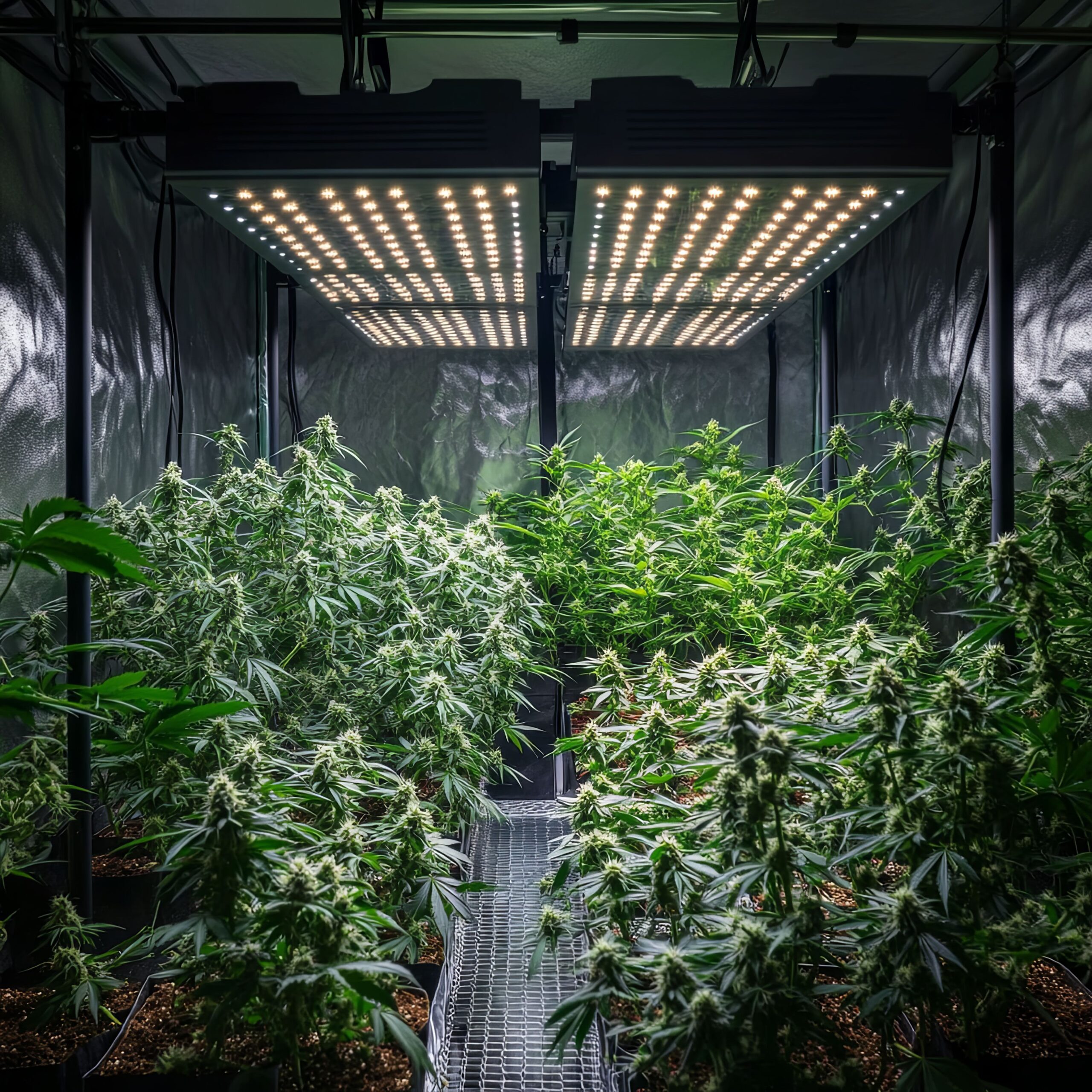
The map’s first job is to show where the photons land. Its second is to summarize whether the occupied crop surface has a broad low zone, a localized high zone, or a workable spread. A colored heatmap without coordinates, dimensions, or actual readings cannot answer those questions reliably. Preserve the raw values and then use visuals to make the spatial pattern easier to see.
Begin by checking the fine print. A credible map identifies the exact fixture or fixture array, operating setting, distance between the light and measurement plane, mapped footprint, point coordinates, sensor methodology, and ideally the surrounding reflective conditions. Find out whether the map includes all fixtures in an array or just one isolated unit. A central PPFD value alone provides none of that context.
Read the map in a fixed sequence. Establish the footprint, identify the centerline, inspect both short and long edges, locate the corners, then trace regions of equal or similar readings. Compare the map to actual plant placement. A low perimeter outside the planted canopy matters differently from a low perimeter holding many flowering branches. The meaning comes from where the values fall relative to the biological crop and the intended design.
Worked example: a 25-point canopy grid
The following 5 × 5 table is a constructed teaching example, not a real experiment or recommended cannabis lighting target. All 25 points are centers of equal-area cells over a hypothetical 100 × 100 cm footprint. Readings are conventional PPFD in µmol/m²/s at one stable horizontal plane under an unchanged fixture setting. The bottom row and side cells are intentionally weaker, with a strong central hotspot.
| Row / column | C1 | C2 | C3 | C4 | C5 |
|---|---|---|---|---|---|
| R1 | 430 | 530 | 580 | 520 | 420 |
| R2 | 540 | 730 | 830 | 710 | 525 |
| R3 | 600 | 850 | 1,010 | 835 | 575 |
| R4 | 520 | 735 | 840 | 720 | 520 |
| R5 | 410 | 520 | 570 | 515 | 405 |
The 25 readings add to 15,440. Because the cells are equal in area, the simple spatial mean is 15,440 ÷ 25 = 617.6 µmol/m²/s. The lowest sampled point is 405; the highest is 1,010. Minimum divided by average is about 0.66, and maximum divided by average is about 1.64. These ratios reveal that a respectable-looking average coexists with a low corner and a center receiving substantially more photon flux. They do not by themselves tell you the optimal correction for a specific crop.
The example exposes two common reporting errors. First, saying “the lamp delivers 1,010 PPFD” describes only one sampled point. Second, saying “the canopy receives 618 PPFD” without reporting the range hides both edge deficit and central intensity. Neither statement is a fair representation of the map by itself. Identify which plants occupy the 400-500 range and which reach near 1,000, then evaluate against your stage-specific plan and the plants’ actual response.
For a basic record, report the mean, minimum, maximum, point count, grid spacing, area, and plane height. The minimum-to-average ratio describes one low extreme relative to the mean. Maximum-to-average highlights a high extreme. The coefficient of variation, calculated as the standard deviation of the grid values divided by their mean, adds information about the overall spread. A histogram or counts within documented bands can reveal whether weak readings are isolated or dominate a substantial part of the footprint.
A peer-reviewed 2022 controlled-environment lighting study demonstrated a limitation of using only minimum divided by average: it does not adequately characterize the distribution above the mean. The authors also considered minimum-to-maximum, a coefficient-of-variation-based measure, and the distribution of normalized readings. The practical consequence is that no single uniformity ratio should become your whole diagnosis. Two maps can share a minimum-to-average value but differ greatly in how much surface is overlit or underlit.
There is no established cannabis-specific universal cutoff at which a map becomes “uniform enough” for every cultivar, stage, lighting economics, and canopy geometry. Choose an operating band from a separate cultivation plan, report the percentage of equally sampled cells within it, inspect the position and magnitude of any outliers, and compare crop response. The zone boundaries must be stated when you display that percentage.
Imagine two fixtures delivering the same 600 PPFD area-average over identical grids. In one, nearly every cell lies between 540 and 660. In the other, the center receives 1,000 while multiple edges sit near 400. Both may produce the same mean, yet tall canopy tops and marginal plants experience very different light conditions. The average represents the overall photon delivery to the sampled plane, not the exposure of every flower.
Conversely, perfectly flat illumination is not the sole objective. Biological light response, fixture efficiency, reflectance, crop placement, and energy cost matter. A small uncovered perimeter can depress minimum-to-average despite the useful planted area receiving fairly even light. That is why the crop footprint must be fixed before calculating statistics, and why a low perimeter should not be discarded merely to improve a number after the fact.
Grower Question
“My average PPFD improved after lowering the fixture, but the outer plants look slower. Should I lower it more?”
Question sent by: Julia Schneider, via contact form.
Not from the average alone. Re-read the same grid and compare minimum, maximum, and the distribution in occupied cells. Lowering can raise the center faster than the edges depending on fixture geometry. Check top-leaf temperature and the condition of edge plants before moving anything again. A higher mean with a worse distribution is not automatically a useful improvement.
Hotspots, weak edges, and false color
A hotspot is a region of unusually high measured PPFD relative to its surroundings. It is not necessarily a diagnosed light injury; a healthy acclimated canopy may use a high value, while heat, drought, or a weak root zone can turn a lower value into a problem. A weak edge may reflect fixture optics, excessive footprint, a single unit placed off-center, plant position, or an incorrectly shaded measurement. Verify unusual values by returning to the same cell before treating them as a physical design problem.
Heatmap colors are a visualization choice. A chart whose red begins at 700 looks more alarming than one whose red begins at 1,200, even when the raw data are identical. Keep the color scale fixed when making before/after comparisons, show its units, and provide the underlying numeric grid. If you use interpolation between widely spaced measurements, label it as estimated surface between sampled points. Do not suggest that colorful smooth contours are directly measured everywhere.
Manufacturer maps versus installed maps
Manufacturer maps answer what was recorded or modeled under their disclosed conditions. An installed map answers what reaches your plane within your actual enclosure, with your wall reflectance, fixture arrangement, plant obstruction, and electrical settings. Differences between the two do not automatically prove marketing deception or meter error. Test height, footprint, boundary sampling, and neighboring-fixture contribution before comparing their averages.
If a chart lacks point values, area, distance, or power setting, treat it as incomplete evidence for a purchase or installation decision. If it shows only a maximum PPFD value, it provides almost no useful information about uniformity. A properly documented installed grid can inform adjustments, but it still does not measure total emitted PPF or verify that an entire crop will yield uniformly.
Pro Tip: Keep two visuals: the unmodified numerical grid and a heatmap drawn from it with a fixed legend. The numerical grid preserves evidence; the heatmap helps you recognize where fixture geometry or plant placement may need attention.
Re-Measure After Every Meaningful Lighting Change
Mapping is most useful as a before/after procedure. The first map establishes the existing spatial pattern. The second tests whether the change solved the actual problem without creating a different one. If you change the hanging height, dimmer, fixture spacing, canopy surface, and photoperiod at once, the result may improve or deteriorate, but you will not know why. Change one controllable variable at a time, preserve the boundary and measurement plane, then repeat the grid.
Height adjustments change distribution as well as intensity
Lowering a fixture usually changes both its photon density at the canopy and the spatial distribution. For a compact point-like source in free space, intensity has an inverse-square relationship with distance under ideal conditions. A wide multi-bar fixture in a reflective tent, however, is not a point source in free space. Treat the inverse-square expression as a concept, not a universal cannabis height calculator. Reflector shape, bar spacing, multiple emission angles, near-field geometry, and wall reflections can invalidate a simple squared-distance prediction.
After lowering the fixture, measure the same 25 cells again with the same operating state and report both maps. The center may gain more than edges, creating a higher maximum-to-average ratio. Raising the fixture may improve distribution in one layout while reducing the mean and increasing spill into unoccupied space. Neither direction is automatically correct; the grid reveals the tradeoff. Stay within the fixture’s mechanical, electrical, cooling, and manufacturer-specified mounting requirements.
Dimming changes output but may not preserve the same pattern
A dimmer setting of 60% is not automatically 60% PPFD. Driver behavior, separate channel controls, spectral changes, and output calibration can make the relationship nonlinear. Measure a stable center reference and a few representative low/high points at each setting you intend to use. If the fixture shape and spectrum stay effectively unchanged, the spatial pattern may scale approximately, but a full repeat grid is needed before claiming that distribution is unchanged.
When changing the photoperiod, don’t use a canopy map to infer daily photons without checking the actual schedule. A dimming ramp, programmable sunrise, or power interruption changes the time integral even if a full-output map looks identical. Keep separate records for spatial distribution and light duration.
Two fixtures introduce a seam where their contributions overlap. An isolated map from fixture A cannot simply be pasted next to the isolated map from fixture B. At each canopy position, total incident PPFD depends on both fixtures, their geometry, the enclosure, and any changed reflectance or obstruction. Under stable conditions, contributions from separate sources can be examined by measuring A only, B only, and both together at the same coordinates, provided the sources can be switched independently and the surroundings stay unchanged. The paired comparison can locate a strong overlap stripe or a dark gap.
Begin with all fixtures in their intended normal operating state. Map the whole planted surface, not individual fixture footprints that hide the seam. If there is a high ridge midway between bars, try one controlled spacing change while preserving safe mounting. If there is a trough, verify whether fixture spacing, height, or the assumed effective area is responsible. A canopy physically spanning the junction needs the combined installed map, not two catalog maps.
Where sources differ in spectrum, ordinary PPFD values can be summed as photon counts only when measured with compatible wavebands and trustworthy source-specific sensor responses. Do not combine an ePPFD figure including far-red with a conventional PPFD figure and call the sum conventional PPFD. Under mixed sunlight and electric light, measure or log the combined environment carefully and avoid treating sequential readings during changing daylight as simultaneous measurements.
What changes when the canopy grows or flowers stretch?
A fixed lamp height above the floor is not a fixed lamp-to-canopy distance. As cannabis stretches, upper leaves rise into a different light field while lower branches may become shaded. Repeat a representative map after major height changes, canopy training, trellis repositioning, pot rearrangement, and installation of new fixtures. Where growth produces an uneven ceiling of flowers, include a separate high-top safety check and note the number of plants outside the main mapped plane.
Do not overinterpret a map made in an empty tent when the growing canopy later occupies much of the enclosure. Plant leaves absorb and redirect light, and the plants themselves block deep zones. Rebuild the relevant map after canopy fill rather than assuming a commissioning measurement remains valid for the whole cycle.
Compare before and after without changing the rules
Use the same coordinates, footprint, sensor, source profile, diffuser if relevant, orientation, door state, and data processing for both surveys. Record the original and revised mean, minimum, maximum, and point-by-point differences. A difference map, calculated as revised PPFD minus original PPFD at each corresponding cell, shows where light was gained or lost. A percentage change can be useful, but a dramatic percentage at a very low baseline may exaggerate practical importance. Keep both absolute and proportional differences available.
A correction is successful only if the desired occupied areas improve without causing unacceptable high exposures elsewhere, violating fixture safety constraints, or increasing energy consumption beyond the intended plan. If the full grid looks better but upper leaves still bleach, revisit leaf temperature, transpiration, root health, spectrum, acclimation, and the possibility that a three-dimensional high point escaped the chosen plane. Measurement improves diagnosis but does not replace observing the crop.
Change one factor at a time
Save the original numeric grid, adjust one variable, stabilize the fixture, repeat the same coordinates, and compare the entire distribution.
Confound every variable
Lowering two lamps, changing the dimmer, opening the enclosure, moving plants, and then presenting one higher center PPFD as proof that uniformity improved.
With the measurement method established, convert only a representative PPFD value into a daily-light estimate.
Convert Measured PPFD Into a Defensible DLI Estimate
PPFD is a rate; daily light integral (DLI) is the cumulative photon dose over a day. A grid shows spatial distribution at the moment and operating setting at which it was collected. To estimate DLI, you must also know the light’s actual time course. For a stable fixture delivering approximately constant PPFD for a known number of hours, a simple calculation is appropriate. For changing sunlight, dimming ramps, or mixed lighting, one snapshot is insufficient.
Convert representative PPFD into a practical DLI estimate
When the light is effectively constant during an operating period, calculate DLI (mol/m²/day) = PPFD (µmol/m²/s) × hours × 0.0036. The factor accounts for 3,600 seconds per hour and one million micromoles per mole. Record the actual operating hours rather than assuming the timer delivered the programmed schedule without interruption.
For the illustrative 25-point map above, average PPFD is 617.6. If the fixture runs at exactly that stable output for 12 hours, its estimated area-average DLI is 617.6 × 12 × 0.0036 = 26.68 mol/m²/day, rounded to two decimals for arithmetic transparency rather than implying laboratory-grade accuracy. At the sampled low corner, 405 × 12 × 0.0036 = 17.50. At the central peak, 1,010 × 12 × 0.0036 = 43.63. These values describe markedly different modeled daily exposures within the same nominal canopy.
Do not report 26.68 as the DLI experienced by every leaf. It is an arithmetic mean across the measured equal-area plane. Interior shaded leaves and unusually tall flowers sit outside that plane, and biological response can differ even where daily totals match. The calculation does not define a universal cannabis target.
Spatial averaging is not temporal averaging
Averaging 25 simultaneous-equivalent locations answers how photons are distributed in space. Averaging repeated readings at one location over the lighting schedule answers how the rate changes over time. These are distinct operations. The appropriate cumulative quantity at a particular position is its time-integrated PPFD; only then can you summarize the daily dose across the mapped area if that is needed.
Suppose one marked point receives 600 PPFD for eight hours and 400 PPFD for four hours, using a documented two-level dimming program. Its illustrative daily total is (600 × 8 + 400 × 4) × 0.0036 = 23.04 mol/m²/day. Multiplying the 600-PPFD peak by 12 hours instead would give 25.92 and overstate this schedule. In reality, sunrise ramps and daylight contributions may vary continuously, requiring appropriately timed logging or integration of recorded measurements.
When a moving sun makes a static grid misleading
In a greenhouse, at a window, or under supplemental grow lighting with significant daylight, the spatial pattern moves as solar angle, clouds, screens, and shadows change. A grid recorded at noon represents noon, not the day. Use logged quantum-sensor data at representative positions or a validated time-sampling procedure to compute location-specific DLI. Report logger interval and missing-data handling. A single spot measurement under a passing cloud cannot be extrapolated into a daily total.
Where the goal is only to quantify supplementary electric lighting, measure it with daylight absent or record separate source contributions under appropriately stable and comparable conditions. Where the goal is plant exposure, the combined photon field is what matters, but you need time-matched data. Avoid subtracting an early-morning daylight value from a late-afternoon combined value and assuming the difference is electric PPFD.
For full unit conversion, reverse calculations, and schedule checks, use the PPFD and DLI Calculator for Cannabis. Here, the relevant limit is simpler: a credible DLI estimate requires both a credible PPFD measurement and the correct time history.
Remember: A PPFD map tells you where photons arrive at one operating condition. DLI adds when and for how long they arrive. Neither converts an inaccurate phone reading into a reliable measurement merely by adding more arithmetic.
Record a Baseline and Troubleshoot From Evidence
One map is useful for installation; a series of consistently collected maps turns light into a measurable cultivation variable. Baselines allow the grower to distinguish a real change in the photon field from a different measurement plane, new sensor, revised fixture setting, or altered canopy shape. They also improve the quality of later diagnosis. A yellow upper leaf alone cannot prove light stress, but its location relative to repeated high PPFD, leaf-temperature measurements, and a documented recent fixture change can narrow the possibilities.
Record a baseline so future light-stress diagnoses are based on data
Store a raw table for each lighting configuration and date. Add one summary line showing area, stage, grid dimensions, mean, minimum, maximum, selected uniformity statistics, photoperiod, and the likely date or plant-height trigger for another survey. Photograph the fixture arrangement and canopy from a consistent viewpoint, but do not substitute a photograph for measured coordinates. Name records consistently, such as Room-A_2026-09-23_5x5_12h, without embedding sensitive personal information or implying that example dates represent real trial data.
Keep a separate plant-response log. At the same crop locations, note leaf temperature where available, air temperature, relative humidity, irrigation events, root-zone condition, discoloration, curling, unusual stretch, and the first date of each symptom. Record which plants are in low, middle, and high exposure regions. When the response differs across the canopy, the spatial pattern can suggest a lighting contribution; when symptoms appear uniformly despite widely different PPFD, investigate additional environmental and root-zone causes.
Diagnose high-top bleaching without assuming PPFD is the only cause
First verify that the suspicious top actually receives more PPFD than nearby healthy tissue by measuring the same orientation and height. Then compare canopy-to-fixture distance, measured leaf temperature, airflow, substrate moisture, and recent changes in light intensity. The top may experience both higher photon flux and higher temperature, especially when different fixture technologies have different radiant-heat behavior. A PPFD meter cannot separate heat injury, drought, nutrient imbalances, or disease by itself.
If the measured light field is unexpectedly high and recent adjustment is plausible, make a conservative, controlled change within the fixture’s safe operating instructions. Preserve a baseline and review the crop over an appropriate observation period before claiming recovery. Existing damaged tissue may not turn green; check unaffected new growth and whether the symptom stops spreading. Do not keep chasing a single printed PPFD number if other environmental variables remain unstable.
Diagnose weak edges and stretched branches
Compare edge readings with the center and with the original map. If a stretch pattern tracks low measured exposure while plant genetics, pruning, crowding, and temperature are otherwise comparable, the lighting distribution becomes a plausible contributor. Correct the coverage geometry, reduce a footprint that exceeds the fixture’s practical reach, or reposition lighting within safe limits, then re-map. Moving plants between zones can blur the evidence; record any deliberate crop rotation and do not describe later differences as caused solely by fixture changes.
Low PPFD is not the only cause of elongated growth. Spectrum, photoperiod, plant density, internode genetics, and temperature can contribute. The map gives you a spatial measurement, not a diagnosis of all morphology.
Recognize when the measurement system, not the lamp, has changed
A sharp discrepancy between two otherwise identical surveys warrants an instrument audit. Confirm the sensor is the same model and calibrated mode, inspect its diffuser, verify the light-source selection and phone software version if relevant, and recheck a reference point. Compare timer and driver logs if available. If possible, make a paired check with a second reliable meter. A global proportional shift might be genuine fixture output loss or a sensor calibration change; a shift confined to one corner suggests geometry, obstruction, plant movement, or transcription error.
Keep uncertainties distinct. Calibration uncertainty concerns the scale of reported PPFD. Repeatability concerns scatter when measuring the same condition repeatedly. Spatial sampling uncertainty concerns what may happen between grid cells. Temporal sampling uncertainty concerns changes during the day or survey. You cannot erase these by reporting extra digits. Increasing grid resolution helps spatial coverage but does not correct a spectrally mismatched sensor; recalibration helps absolute readings but does not reconstruct missing sunlight history.
Set a re-measurement trigger, not an arbitrary calendar ritual
Useful triggers include a fixture move, driver or lamp replacement, meaningful dimming change, major increase in canopy height, change in planted footprint, unusual edge growth, suspected hotspot, altered reflective surfaces, or significant daylight-season shift for a greenhouse. Add a scheduled periodic check appropriate to the operation and instrument maintenance plan, but verify the event that actually changed the physical light field. A new map every day under an unchanged stable light might generate more data than value, while a single map for an entire flowering cycle can miss major canopy-height changes.
Grower Question
“Can I use last month’s PPFD map if the fixture has not moved?”
Question sent by: MapleGrower, via Facebook page.
Only as a historic reference. If plants have grown toward the light, a trellis has changed canopy height, pots have moved, or a driver setting has changed, the old map no longer represents the same plane or configuration. Repeat the appropriate measurement, record what changed, and compare only the corresponding areas.
Use map evidence without turning correlations into cultivar claims
A higher-yielding plant under a higher measured PPFD does not prove the higher PPFD alone produced the difference. Position can also affect airflow, temperature, irrigation delivery, genetics, plant size, and training history. Controlled cannabis lighting research measures canopy PPFD and adjusts fixture height repeatedly to preserve treatment conditions; its results still depend on cultivar, spectrum, and the experimental environment. For a production comparison, document those confounders and use replication rather than reading causality from one productive corner.
Similarly, a map showing that two fixtures achieve the same mean does not prove equivalent energy efficiency. Compare measured electrical input, PPF/PPE from credible testing, area covered, and the useful distribution, then assess crop performance separately. The indoor growing basics guide provides general system context, while this page remains focused on the measurement procedure.
Verify Your Measurement and Make the Next Decision
A usable PPFD map lets another person reproduce the measurements and reach the same descriptive result within known instrument and environmental uncertainty. It should also tell you what action follows. The final review below separates a trustworthy measurement from an attractive chart and keeps adjustment decisions proportional to the evidence.
Audit the map before interpreting it
Ask whether the grid covers the declared planted area, whether cells are equal in area or correctly weighted, and whether all readings represent one documented plane and operating state. Inspect the raw values for missing coordinates, duplicated entries, a misplaced row, an implausible sensor reading, and an unrecorded change in room light. Return to suspect cells. If a reference point changed during the survey, stabilize the setup and repeat rather than burying drift inside the average.
Choose the next action from the measured failure
| Observed evidence | Next check | Controlled action and verification |
|---|---|---|
| High center; weak perimeter | Confirm area, plane, height, and edge occupancy | Test an allowable height or distribution change; repeat the identical grid. |
| High seam under two fixtures | Compare whole-array and, if safe, individual-source contributions | Test spacing or output balance one change at a time; re-map the overlap. |
| App and quantum meter disagree | Compare sensor mode, diffuser, spectrum profile, and reference points | Use traceable/reference reading for absolute decisions; treat unresolved app values as estimates. |
| Grid differs on identical repeat | Check drift, shading, warm-up, sensor condition, and transcription | Re-stabilize and resurvey; do not interpret unstable readings as crop conditions. |
| Good average; injured tallest top | Measure that top separately; inspect leaf temperature and root zone | Correct a verified exposure/environmental problem and monitor unaffected growth. |
| Stable PPFD but altered photoperiod | Verify actual timer output and ramps | Recalculate DLI from time history; do not assume the daily dose is unchanged. |
| Greenhouse points vary during the survey | Log reference PPFD and sky/screens over time | Use synchronized or appropriately time-integrated measurements before spatial claims. |
Pre-adjustment and final verification checklist
Final measurement check
Repeatable canopy-light measurement checklist
- State the question: absolute PPFD, spatial uniformity, before/after correction, or DLI estimate.
- Define the planted footprint, coordinate system, grid spacing, and representative canopy plane.
- Check meter type, PAR/ePAR waveband, serial ID, calibration, optical cleanliness, and sensor orientation.
- If using a phone, record device, app, sensing mode, spectrum profile, diffuser, and reference-validation status.
- Document fixture layout, operating settings, height, timer, warm-up state, enclosure, and canopy geometry.
- Take every cell reading without self-shading; preserve the raw values and revisit suspect points.
- Repeat a fixed reference reading at the end and resolve meaningful drift.
- Report mean, minimum, maximum, point count, location of weak/high regions, and distribution information.
- Use actual operating hours or logged PPFD over time before calling an estimate DLI.
- Make one safe change, repeat the identical grid, and evaluate both plant response and the new spatial pattern.
Where to go after the map
Once you know the installed distribution, the next question is whether the measured photon exposure suits the crop’s stage, environment, and production objective. This page does not supply a universal stage target. Use Cannabis PPFD and DLI by Growth Stage for stage context and the PPFD and DLI Calculator for schedule calculations. For broad fixture choice, electrical sizing, and indoor system considerations, the established grow lights pillar remains the parent reference.
Bottom line: a credible canopy map is a documented measurement of a defined surface, not a center reading or an app screenshot. Keep the geometry, sensor, spectrum, and operating state consistent, use the complete distribution rather than the mean alone, and verify each change with the same grid. That is how light measurements become an actionable grow-room baseline rather than another uncertain number.
Share this article
A quick overview of the topics covered in this article.
Follow us
Latest articles
October 3, 2026